The First-order Integer-valued Autoregressive (INAR(1)) model with zero-inflated (ZI-INAR(1)) and hurdle (H-INAR(1)) innovations is widely used in studying integer-valued time-series data, such as crime count and heatwave frequency. This work implemented the INAR(1) models in Stan.
You can install ZIHINAR1 from GitHub with:
remotes::install_github("fushengyy/ZIHINAR1")\[Available Soon\] Or you can install the released version of HeckmanStan from CRAN with:
install.packages("ZIHINAR1")The package contains main function named get_stanfit().
stan_fit <- get_stanfit(mod_type, distri, y, n_pred = 4,
                        thin = 2, chains = 1, iter = 2000, warmup = iter/2,
                        seed = NA)
mod_type: Character string indicating the model type. Use “zi” for zero-inflated models and “h” for hurdle models.
distri: Character string specifying the distribution. Options are “poi” for Poisson or “nb” for Negative Binomial.
y: A numeric vector of integers representing the observed data.
n_pred: Integer specifying the number of time points for future predictions (default is 4).
thin: Integer indicating the thinning interval for Stan sampling (default is 2).
chains: Integer specifying the number of Markov chains to run (default is 1).
iter: Integer specifying the total number of iterations per chain (default is 2000).
warmup: Integer specifying the number of warmup iterations per chain (default is iter/2).
seed: Numeric seed for reproducibility (default is NA).
The following are examples showing how to fit the INAR(1) model when data is generated from a zero-inflated Negative Binomial (ZINB) distribution.
library(ZIHINAR1)
y_data <- data_simu(n = 100, alpha = 0.5, rho = 0.3, theta = c(5, 2),
mod_type = "zi", distri = "nb")
stan_fit <- get_stanfit(mod_type = "zi", distri = "nb", y = y_data, n_pred = 5,
iter = 2000, chains = 1, warmup = 500,
thin = 2, seed = 42)
#>
#> SAMPLING FOR MODEL 'anon_model' NOW (CHAIN 1).
#> Chain 1:
#> Chain 1: Gradient evaluation took 0.002477 seconds
#> Chain 1: 1000 transitions using 10 leapfrog steps per transition would take 24.77 seconds.
#> Chain 1: Adjust your expectations accordingly!
#> Chain 1:
#> Chain 1:
#> Chain 1: Iteration: 1 / 2000 [ 0%] (Warmup)
#> Chain 1: Iteration: 200 / 2000 [ 10%] (Warmup)
#> Chain 1: Iteration: 400 / 2000 [ 20%] (Warmup)
#> Chain 1: Iteration: 501 / 2000 [ 25%] (Sampling)
#> Chain 1: Iteration: 700 / 2000 [ 35%] (Sampling)
#> Chain 1: Iteration: 900 / 2000 [ 45%] (Sampling)
#> Chain 1: Iteration: 1100 / 2000 [ 55%] (Sampling)
#> Chain 1: Iteration: 1300 / 2000 [ 65%] (Sampling)
#> Chain 1: Iteration: 1500 / 2000 [ 75%] (Sampling)
#> Chain 1: Iteration: 1700 / 2000 [ 85%] (Sampling)
#> Chain 1: Iteration: 1900 / 2000 [ 95%] (Sampling)
#> Chain 1: Iteration: 2000 / 2000 [100%] (Sampling)
#> Chain 1:
#> Chain 1: Elapsed Time: 3.767 seconds (Warm-up)
#> Chain 1: 9.449 seconds (Sampling)
#> Chain 1: 13.216 seconds (Total)
#> Chain 1:
get_est(distri = "nb", stan_fit = stan_fit)
#>
#>
#> Table: Parameter Estimates
#>
#> Mean SD Median Q2.5 Q97.5 Rhat 95%_HPD_Lower 95%_HPD_Upper
#> ------- ------- ------- ------- ------- ------- ------- -------------- --------------
#> alpha 0.5434 0.0407 0.5450 0.4620 0.6123 1.0010 0.4605 0.6113
#> rho 0.2573 0.1131 0.2506 0.0404 0.4742 1.0006 0.0437 0.4753
#> lambda 4.9955 0.7772 4.9750 3.6025 6.5105 0.9987 3.6044 6.5105
#> phi 2.2278 1.2160 1.9962 0.7745 4.9245 0.9993 0.5618 4.3624
get_mod_sel(y = y_data, mod_type = "zi", distri = "nb", stan_fit = stan_fit)
#>
#>
#> Table: Model Selection Criteria
#>
#> EAIC EBIC DIC WAIC1 WAIC2
#> --------- --------- --------- --------- ---------
#> 554.6341 565.0146 555.8627 550.0862 550.3367
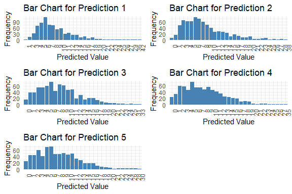
get_pred(stan_fit = stan_fit)
#>
#>
#> Table: Summary of Predictions
#>
#> Mode Median IQR Min Max
#> --------- ----- ------- ---- ---- ----
#> y_pred.1 6 7.0 5 1 42
#> y_pred.2 6 7.0 7 0 38
#> y_pred.3 6 7.5 7 0 33
#> y_pred.4 5 7.0 7 0 35
#> y_pred.5 6 7.0 7 0 30